This Simple 2009 Strategy Still Wins 75% of the Time
The same rules worked on ES and 10 Year Notes. Volatility matched, the two models produced a 2.61 profit factor, negative 0.08 correlation and 23.59 Return/DD.

Simple trading ideas are easy to dismiss.
This one has been public since 2009.
It trades a basic mean reversion pattern on daily bars. No complicated indicator stack. No machine learning. No market specific rewrite.
On ES, the strategy produced:
$134,800 net profit
74.41% winning trades
2.48 profit factor
$638.86 average trade
I then applied the same rules to TY, the 10 Year US Treasury Note futures market.
The TY version produced:
$214,218.75 net profit
75.79% winning trades
2.71 profit factor
$1,127.47 average trade
Both markets produced strong standalone results.
But the better result came from combining them.
After sizing TY to roughly match the dollar volatility of ES, the combined portfolio produced:
$349,018.80 total profit
75.06% winning trades
2.61 profit factor
$14,796.87 maximum drawdown
23.59 Return/DD
Negative 0.08 correlation
The profits added together.
The drawdowns did not.
That is what makes this simple strategy useful beyond the standalone backtest.
It becomes a portfolio building block.
Most of the Results Came After Publication
The strategy comes from Larry Connors and Cesar Alvarez’s 2009 book, High Probability ETF Trading.
The publication date gives us something valuable: a long period of genuine unseen data.
The ES test begins in 1997.
The TY test begins in 2001.
More than half of the ES results and roughly two thirds of the TY results occurred after the strategy was already public.
The rules were fixed before:
The long low rate period
The COVID crash
The inflation surge
The 2022 stock and bond decline
The rate increase cycle
The markets that followed
This does not guarantee the edge will continue.
It does make the test more meaningful than creating a strategy today using the entire historical record.
The rules came first.
Most of the data came later.
The edge survived.
ES Results Since 1997
The first test uses ES daily bars.
At a high level, the model looks for a short term price pattern that has moved too far against the broader trend.
It trades both long and short.
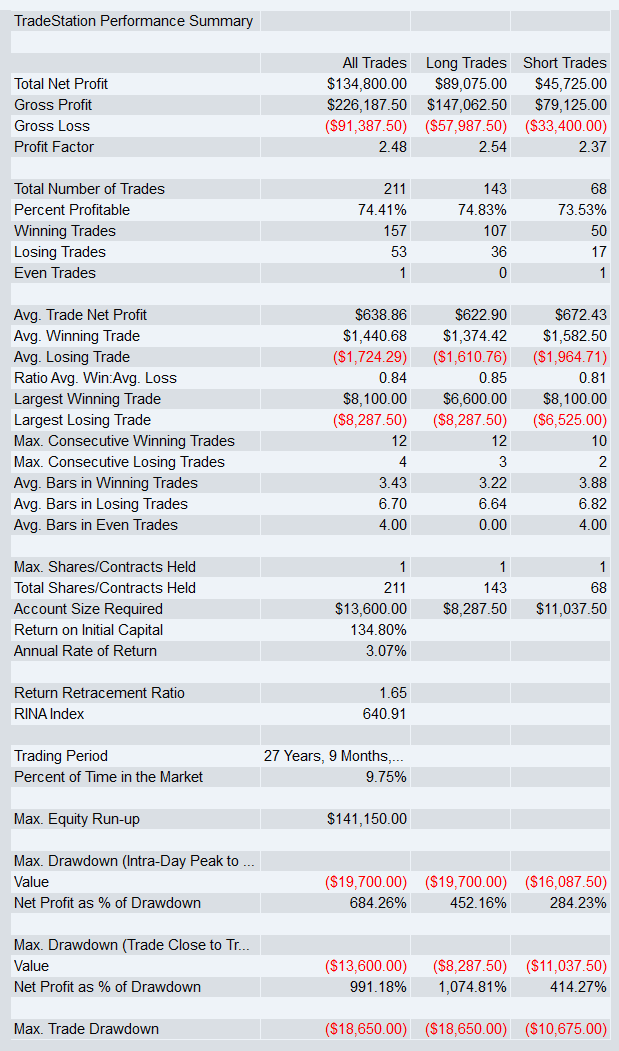
ES performance
A win rate near 75% looks good, but win rate alone means very little.
It needs to be supported by profit factor, average trade and drawdown.
Here, the strategy produced $2.48 in gross profit for every $1 in gross losses. The average trade was also large enough to leave room for realistic trading costs.
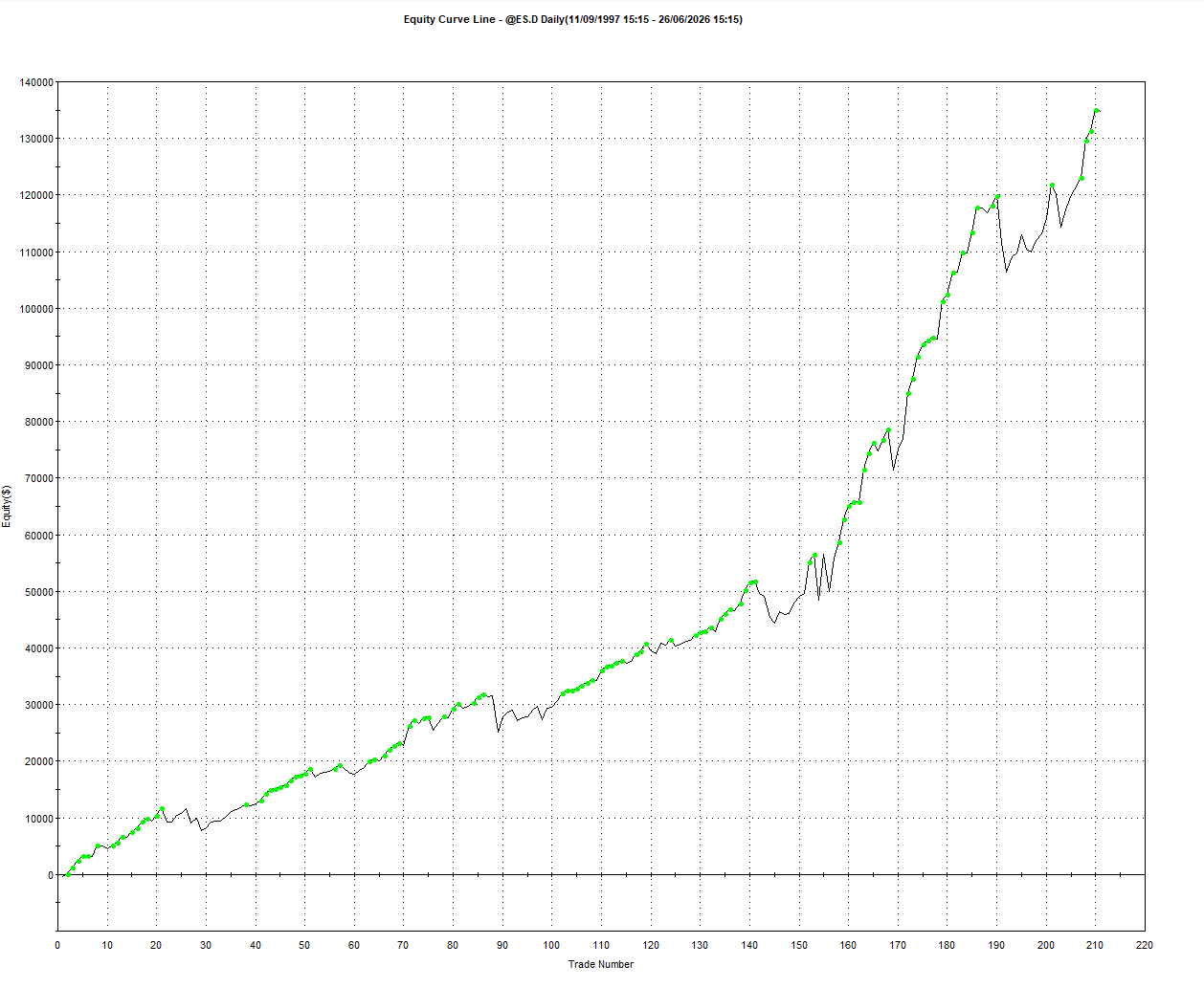
The equity curve is not perfect.
There are drawdowns and flat periods. That is normal across nearly three decades of testing.
The important point is that the strategy continued making new highs across very different equity market regimes.
ES monthly performance
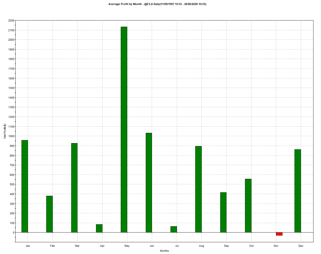
The ES model was profitable on average in 11 of the 12 calendar months.
May was the strongest month, followed by June, January and March.
November was the only slightly negative month.
The edge was not dependent on one small seasonal window.
TY Results Since 2001
The second test applies the same rules to TY.
This is a better robustness test than moving from ES to another equity index.
Treasury futures are driven by different forces:
Interest rates
Inflation expectations
Federal Reserve policy
Economic growth
Defensive capital flows
If the strategy only captured an equity specific behaviour, it should have weakened when moved to bonds.
It did not.
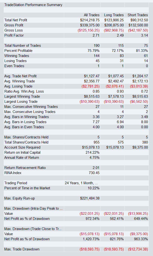
TY performance
TY produced a slightly higher win rate, profit factor and Return/DD than ES.
The short side also made a real contribution:
$90,312.50 net profit
81.33% winning trades
3.14 profit factor
75 short trades
This matters because bonds went through a major bear market as interest rates increased.
The strategy was not forced to remain long throughout that decline.
It could trade short when the broader regime turned bearish.
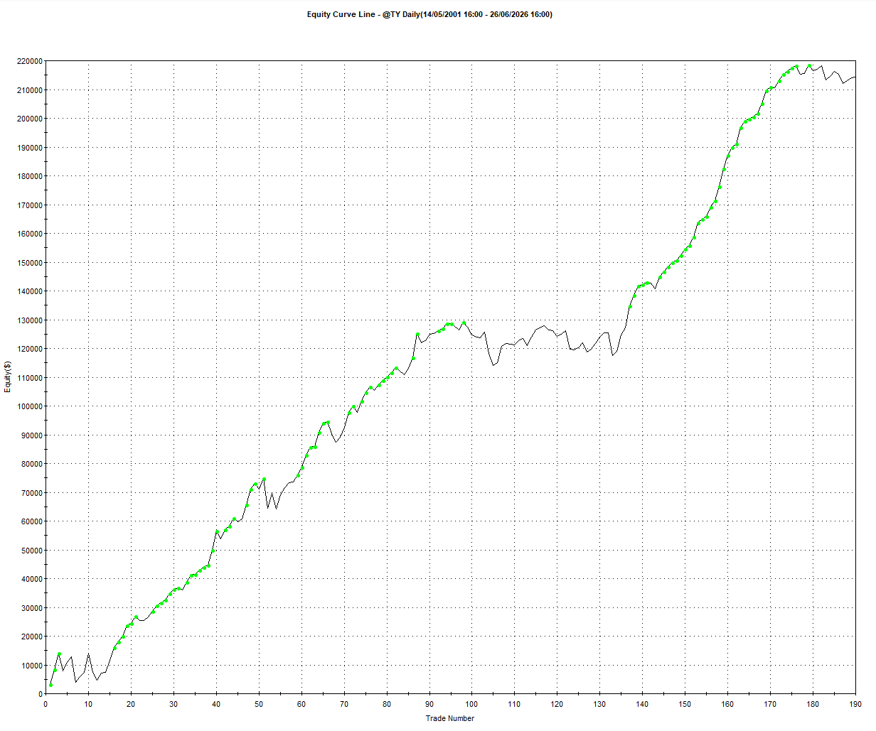
The TY equity curve had its own difficult periods.
Those periods did not always occur at the same time as the ES drawdowns.
That becomes important when the two markets are combined.
TY monthly performance
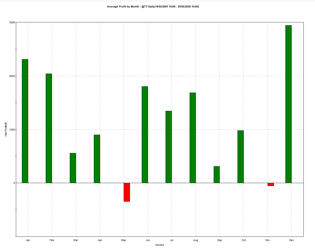
The monthly profile was also different from ES.
December was the strongest TY month, followed by January and February.
May and November were the only negative average months.
The different monthly profiles are another sign that the two systems are not producing the same return stream.
Why Combine Stocks and Bonds?
The traditional 60/40 portfolio became popular because stocks and bonds have historically responded to different economic forces.
Stocks are driven heavily by earnings, growth, liquidity and risk sentiment.
Government bonds are driven more by interest rates, inflation and monetary policy.
Because the drivers are different, stocks and bonds have often experienced their strongest and weakest periods at different times.
That can make the combined portfolio smoother than either asset held alone.
I am not recreating a 60/40 allocation here.
The contract mix is not 60% ES and 40% TY.
I am taking the principle that made the stock and bond combination popular and applying it to short term systematic trading:
Combine return streams that do not struggle at the same time.
The same trading logic is used on both markets.
The return drivers are different.
That produced a strategy correlation of:
Negative 0.08

Negative 0.08 is not a strong inverse relationship.
It does not need to be.
The goal is not for one strategy to rise every time the other falls.
The goal is to avoid having both strategies lose together consistently.
That is exactly what the test shows.
Matching the Volatility
One ES contract and one TY contract do not carry the same dollar volatility.
Trading one contract of each would make the portfolio look diversified, but ES would still control most of the movement.
To make the comparison more balanced, the TY position was increased to roughly match the dollar volatility of one ES contract.
The test uses:
1 ES contract
5 TY contracts
This is not a 60/40 capital allocation.
It is a simple volatility matching method.
The goal is to give both return streams enough weight to matter without allowing one market to dominate the portfolio.
A live implementation could update this more dynamically using ATR, rolling dollar volatility or expected drawdown contribution.
For this test, the fixed contract ratio keeps the comparison simple.
The Combined Portfolio
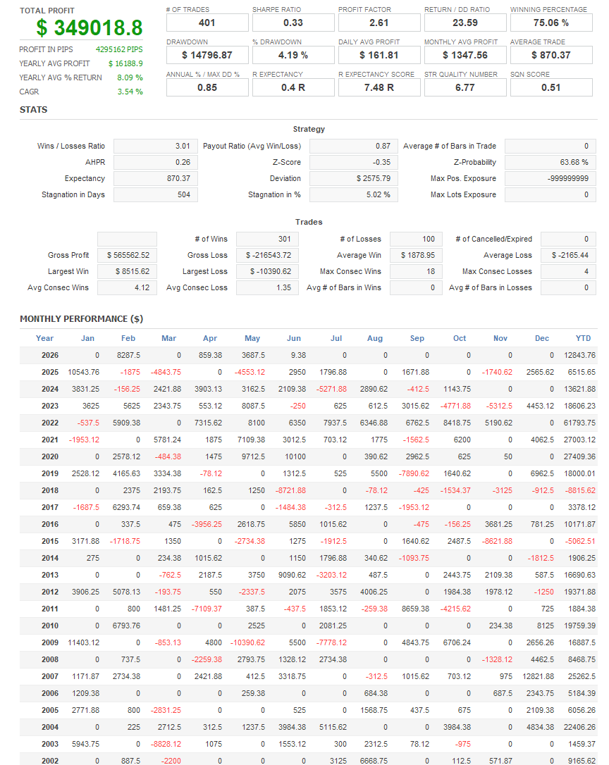
This is the payoff.
The combined portfolio produced almost the full sum of both strategy profits.
But maximum drawdown did not double.
Compared with ES alone, the portfolio produced around 2.59 times the profit, while drawdown increased by only about 8.8%.
Compared with TY alone, the portfolio produced around 1.63 times the profit, while maximum drawdown was slightly lower.
Return/DD improved to 23.59.
That is:
Around 138% higher than ES
Around 66% higher than TY
Return/DD measures how much total profit the strategy produced relative to its largest historical drawdown.
Higher is better.
Profit can always be increased by adding more contracts. That does not make the strategy more efficient.
Here, the improvement came from combining two return streams that did not lose at the same time.
Combined equity curve
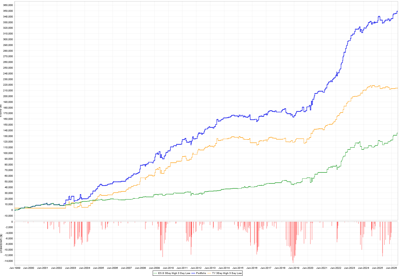
The blue line is the combined portfolio.
The orange and green lines are the individual TY and ES strategies.
The portfolio still has drawdowns.
It still has flat periods.
But the path is more consistent because the portfolio is not dependent on one market environment.
The combined maximum stagnation was 504 days.
The strategy is strong on each market.
The low correlation makes it stronger as a portfolio.
